Hi! I' am Pedro Henrique Braga Moraes and this work is a part of the digital image processing course ministered by professor Agostinho de Medeiros Brito, at UFRN. Here you will find a lot of OpenCV and jojo’s references.
1. Manipulating pixels in an image
1.1. Negative
This first program basicaly asks the cordinates from the user and take the negative of the rectangular region. The algorithm converts the image to grayscale and for each pixel in the region it makes 255 - (value of the pixel).
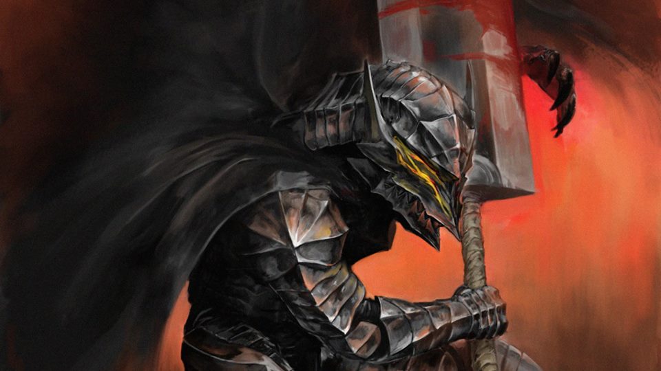
Berserk.jpg before negative:
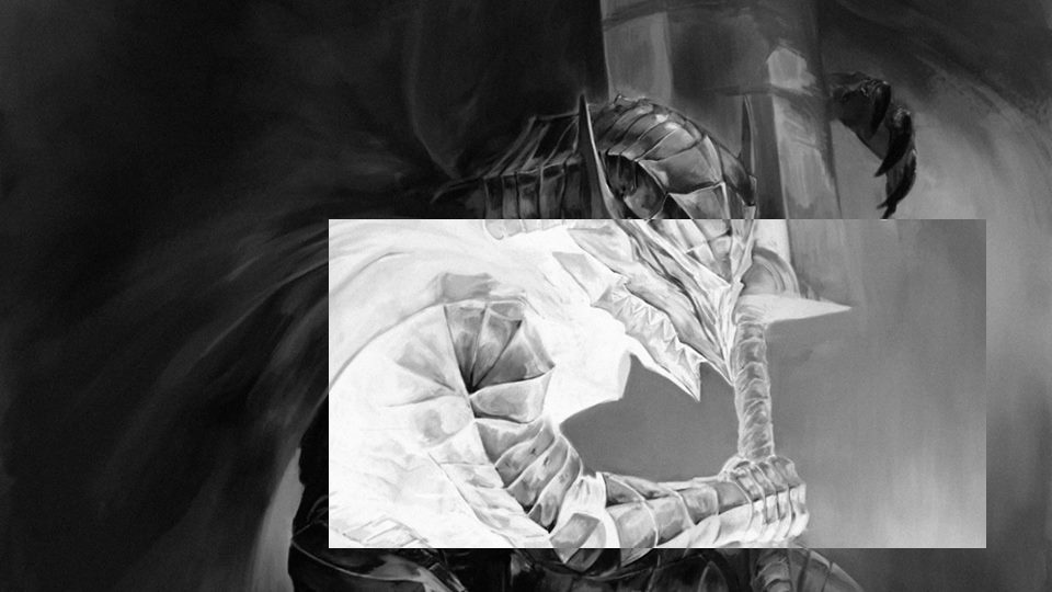
Berserk.jpg after negative:
#include <iostream>
#include <opencv2/opencv.hpp>

using namespace cv;
using namespace std;


int main(int, char**){
  int X1, X2, Y1, Y2;
  Mat image;
  Vec3b val;

  do{
  cout<<"Digite o valor de X1:  ";
  cin >> X1;
  cout << endl;
  if (X1>960 || X1<0)
    cout << "Numero fora da faixa! Digite outro! ";
    cout << endl;}
  while (X1>960 || X1<0);

  do{
  cout<<"Digite o valor de X2:  ";
  cin >> X2;
  cout << endl;
  if (X2>960 || X2<0)
    cout << "Numero fora da faixa! Digite outro! ";
    cout << endl;}
  while (X2>960 || X2<0);


  do{
  cout<<"Digite o valor de Y1:  ";
  cin >> Y1;
  cout << endl;
  if (Y1>540 || Y1<0)
    cout << "Numero fora da faixa! Digite outro! ";
    cout << endl;}
  while (Y1>540 || Y1<0);


  do{
  cout<<"digite o valor de Y2:  ";
  cin >> Y2;
  cout << endl;
  if (Y2>540 || Y2<0)
    cout << "Numero fora da faixa! Digite outro! ";
    cout << endl;}
  while (Y2>540 || Y2<0);


  image= imread("berserk.jpg",CV_LOAD_IMAGE_GRAYSCALE);
  if(!image.data)
    cout << "nao abriu berserk.jpg" << endl;

  namedWindow("janela",WINDOW_AUTOSIZE);

  for(int j=X1;j<X2;j++){ // eixo x e y invertidos, y é o eixo horizontal e x o vertical
    for(int i=Y1;i<Y2;i++){
       image.at<uchar>(i, j) =  255 - image.at<uchar>(i, j);
    }
  }

  imshow("janela", image);
  //imwrite("negativo.jpg", image);

  waitKey();
  return 0;
}
1.2. Swapping regions
This code divides the image in 4 quadrants and swaps the regions.
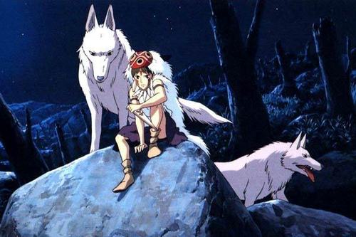
mononoke.jpg before swap:
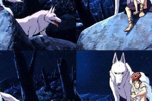
mononoke.jpg after swap:
#include <iostream>
#include <opencv2/opencv.hpp>

using namespace cv;
using namespace std;


int main(int, char**){

  Mat image;
  image = imread("mononoke.jpg");
  int r = image.rows;
  int mr = image.rows/2;
  int c = image.cols;
  int mc = image.cols/2;
  Mat vazia = Mat::zeros(r, c, CV_8UC3);
  if(!image.data)
    cout << "nao abriu a imagem!" << endl;

  namedWindow("trocada", WINDOW_AUTOSIZE);

  for(int j=0;j<c;j++){
    for(int i=0;i<r;i++)

      {
         if(i < mr && j < mc)
            vazia.at<Vec3b>(i, j) =  image.at<Vec3b>(i+mr, j+mc);
         if(i > mr && j > mc)
         	vazia.at<Vec3b>(i, j) =  image.at<Vec3b>(i-mr, j-mc);
         if(i > mr && j < mc)
         	vazia.at<Vec3b>(i, j) =  image.at<Vec3b>(i-mr, j+mc);
         if(i < mr && j > mc)
         	vazia.at<Vec3b>(i, j) =  image.at<Vec3b>(i+mr, j-mc);
      }

  }

  imshow("trocada", vazia);
  imwrite("trocada.jpg", vazia);

  waitKey();
  return 0;
}
2. Objects couting
2.1. Labeling
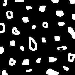
This program counts the objects in the image, differentiating the ones with and without holes.
First we have the image:
#include <iostream>
#include <opencv2/opencv.hpp>
using namespace cv;
using namespace std;
int main(int argc, char** argv){
Mat image, mask;
int c, r, total = 0, hole = 0;
CvPoint p;
image = imread(argv[1],CV_LOAD_IMAGE_GRAYSCALE);
if(!image.data){
std::cout << "imagem nao carregou corretamente\n";
return(-1);
}
c=image.cols;
r=image.rows;
p.x=0;
p.y=0;
for(int i=0; i<r; i++){
for(int j=0; j<c; j++){
if(image.at<uchar>(i,j) == 255){
if(i == 0 || j == 0 || i == (r-1) || j == (c-1) ){
p.x=j;
p.y=i;
floodFill(image,p, 0);}
}
}
}
p.x = 0;
p.y = 0;
floodFill(image, p, 200);
for(int i=0; i<r; i++){
for(int j=0; j<c; j++){
if(image.at<uchar>(i,j) == 255){
p.x=j;
p.y=i;
total++;
//colour1++;
floodFill(image, p, 30);
}}}
imshow("image", image);
imwrite("bolhas1.png", image);
waitKey();
for(int i=0; i<r; i++){
for(int j=0; j<c; j++){
if(image.at<uchar>(i,j) == 0){
if(image.at<uchar>(i-1,j) != 200){
hole++;
p.x=j;
p.y=i;
floodFill(image, p, 200);
p.x=j;
p.y=i-1;
floodFill(image, p, 200);}
else
p.x=j;
p.y=i;
floodFill(image,p, 200);
}}}
imshow("image", image);
imwrite("labeling.png", image);
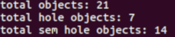
cout << "total objects: " << total <<endl;
cout << "total hole objects: " << hole <<endl;
cout << "total sem hole objects: " << total - hole <<endl;
waitKey();
return 0;
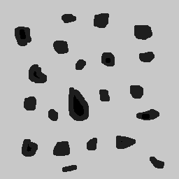
}After running the program, the first thing that happens is deleting the objects that touch the boarder:
Then the counting can happen:
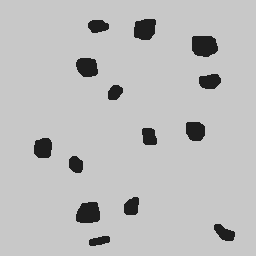
Results:
It’s worth poiting out that this programs works also with images that have objects with two or more holes.
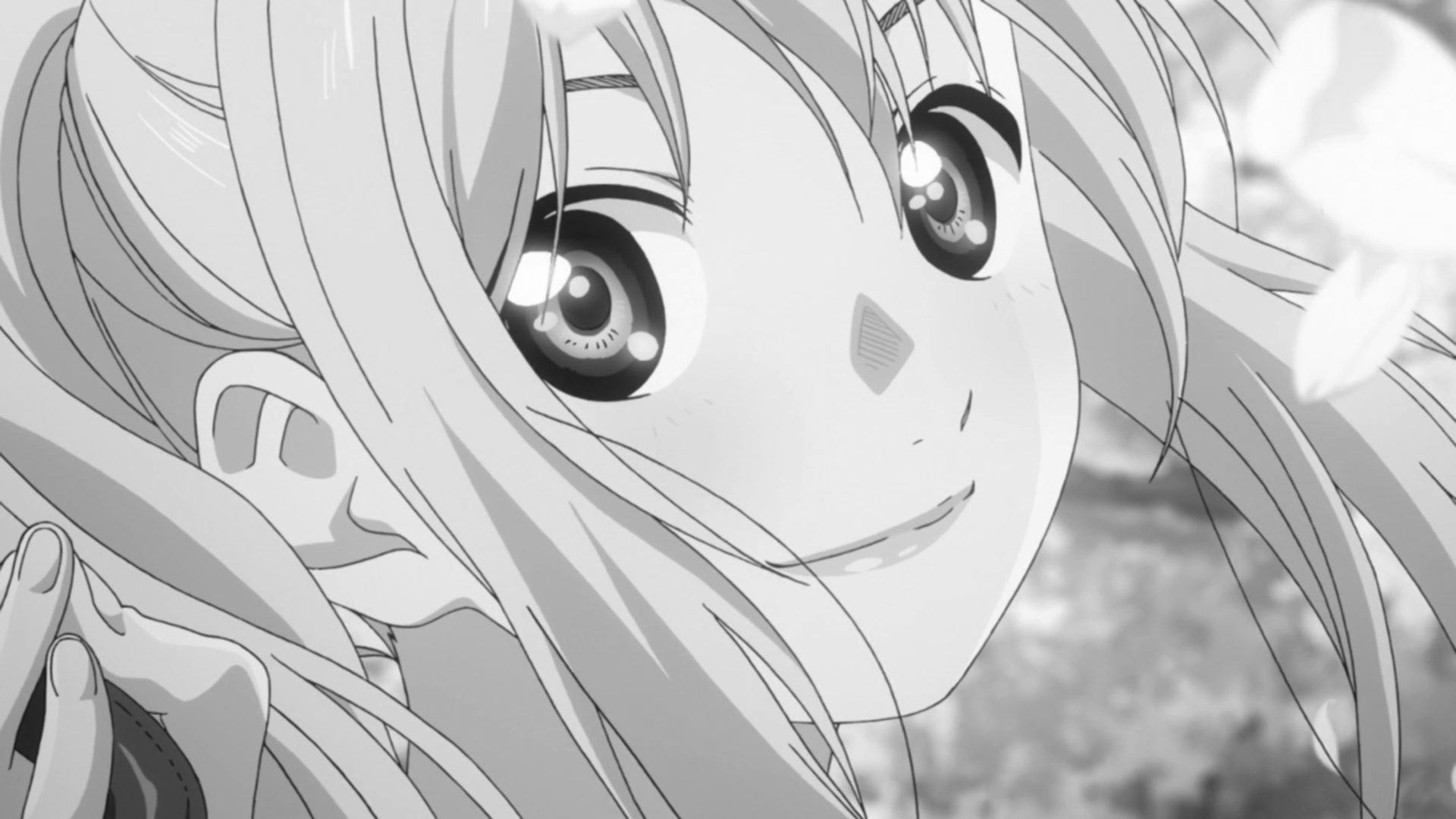
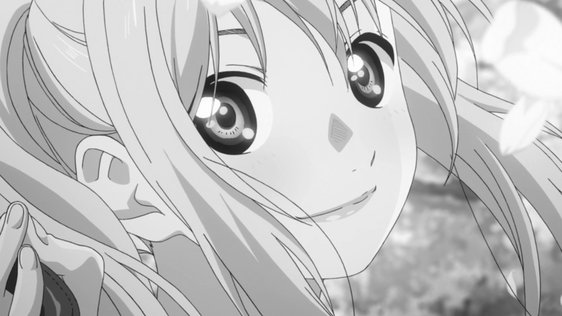
3. Histograms
3.1. Equalize image
The algorithm below equilizes and shows the image’s histogram.
Original image:
#include <iostream>
#include <opencv2/opencv.hpp>

using namespace cv;
using namespace std;

int main(int argc, char** argv){

Mat img, img_eq, hist, hist_eq;
int nbins = 64;

float range[] = {0, 256};
const float *histrange = { range };

img= imread("nice.jpg",CV_LOAD_IMAGE_GRAYSCALE);
  if(!img.data)
    cout << "nao abriu nice.jpg" << endl;

equalizeHist( img, img_eq );


bool uniform = true;
bool acummulate = false;

int histw = nbins, histh = nbins / 2;
Mat hist_img(histh, histw, CV_8UC1, Scalar(0, 0, 0));
Mat hist_img_eq(histh, histw, CV_8UC1, Scalar(0, 0, 0));

calcHist(&img, 1, 0, Mat(), hist, 1, &nbins, &histrange, uniform, acummulate);
calcHist(&img_eq, 1, 0, Mat(), hist_eq, 1, &nbins, &histrange, uniform, acummulate);

normalize(hist, hist, 0, hist_img.rows, NORM_MINMAX, -1, Mat());
normalize(hist_eq, hist_eq, 0, hist_img.rows, NORM_MINMAX, -1, Mat());

hist_img.setTo(Scalar(0));
hist_img_eq.setTo(Scalar(0));

for(int i=0; i<nbins; i++){
  line(hist_img, Point(i, histh), Point(i, 32 - cvRound(hist.at<float>(i))), Scalar(255, 255, 255), 1, 8, 0);
  line(hist_img_eq, Point(i, histh), Point(i, 32 - cvRound(hist_eq.at<float>(i))), Scalar(255, 255, 255), 1, 8, 0);}

hist_img.copyTo(img(Rect(15, 15, nbins, histh)));
hist_img_eq.copyTo(img_eq(Rect(15, 15, nbins, histh)));


namedWindow("nice",WINDOW_AUTOSIZE);
namedWindow("equilised_nice",WINDOW_AUTOSIZE);


imshow( "nice", img );
imshow( "equalised_nice", img_eq );
imwrite("nice_hist.jpg", img);
imwrite("nice_equilised_hist.jpg", img_eq);

waitKey();
return 0;}
The output, jojo and the histogram:
Jojo and the equalized histogram:

3.2. Equalize video
The same process, but now with a video of an amazing spear fight:
#include <iostream>
#include <opencv2/opencv.hpp>

using namespace cv;
using namespace std;

int main(int argc, char** argv){

Mat img, img_eq, hist, hist_eq;
int nbins = 64;

float range[] = {0, 256};
const float *histrange = { range };

VideoCapture cap("barca.mp4");
  if(!cap.isOpened()){
    cout << "Erro abrindo o video!" <<endl;
    return -1;
  }
int width  = cap.get(CV_CAP_PROP_FRAME_WIDTH);
int height = cap.get(CV_CAP_PROP_FRAME_HEIGHT);
//VideoWriter video1("barca.avi",CV_FOURCC('P','I','M','1'),30, Size(width, height),0);
//VideoWriter video2("barca_eq.avi",CV_FOURCC('P','I','M','1'),30, Size(width, height),0);
while(1){
    cap >> img;
    if (img.empty())
     	break;
cvtColor(img, img, CV_BGR2GRAY);
equalizeHist( img, img_eq );


bool uniform = true;
bool acummulate = false;

int histw = nbins, histh = nbins / 2;
Mat hist_img(histh, histw, CV_8UC1, Scalar(0, 0, 0));
Mat hist_img_eq(histh, histw, CV_8UC1, Scalar(0, 0, 0));

calcHist(&img, 1, 0, Mat(), hist, 1, &nbins, &histrange, uniform, acummulate);
calcHist(&img_eq, 1, 0, Mat(), hist_eq, 1, &nbins, &histrange, uniform, acummulate);

normalize(hist, hist, 0, hist_img.rows, NORM_MINMAX, -1, Mat());
normalize(hist_eq, hist_eq, 0, hist_img_eq.rows, NORM_MINMAX, -1, Mat());

hist_img.setTo(Scalar(0));
hist_img_eq.setTo(Scalar(0));

for(int i=0; i<nbins; i++){
  line(hist_img, Point(i, histh), Point(i, 32 - cvRound(hist.at<float>(i))), Scalar(255, 255, 255), 1, 8, 0);
  line(hist_img_eq, Point(i, histh), Point(i, 32 - cvRound(hist_eq.at<float>(i))), Scalar(255, 255, 255), 1, 8, 0);}

hist_img.copyTo(img(Rect(15, 15, nbins, histh)));
hist_img_eq.copyTo(img_eq(Rect(15, 15, nbins, histh)));


//video1.write(img);
//video2.write(img_eq);
namedWindow("nice",WINDOW_AUTOSIZE);
namedWindow("equilised_video",WINDOW_AUTOSIZE);


if (img.empty())
     	break;

imshow( "video", img );
imshow( "equalised_video", img_eq );
if(waitKey(30) >= 0)
    	break;
}
cap.release();
destroyAllWindows();


waitKey();
return 0;}
The output:
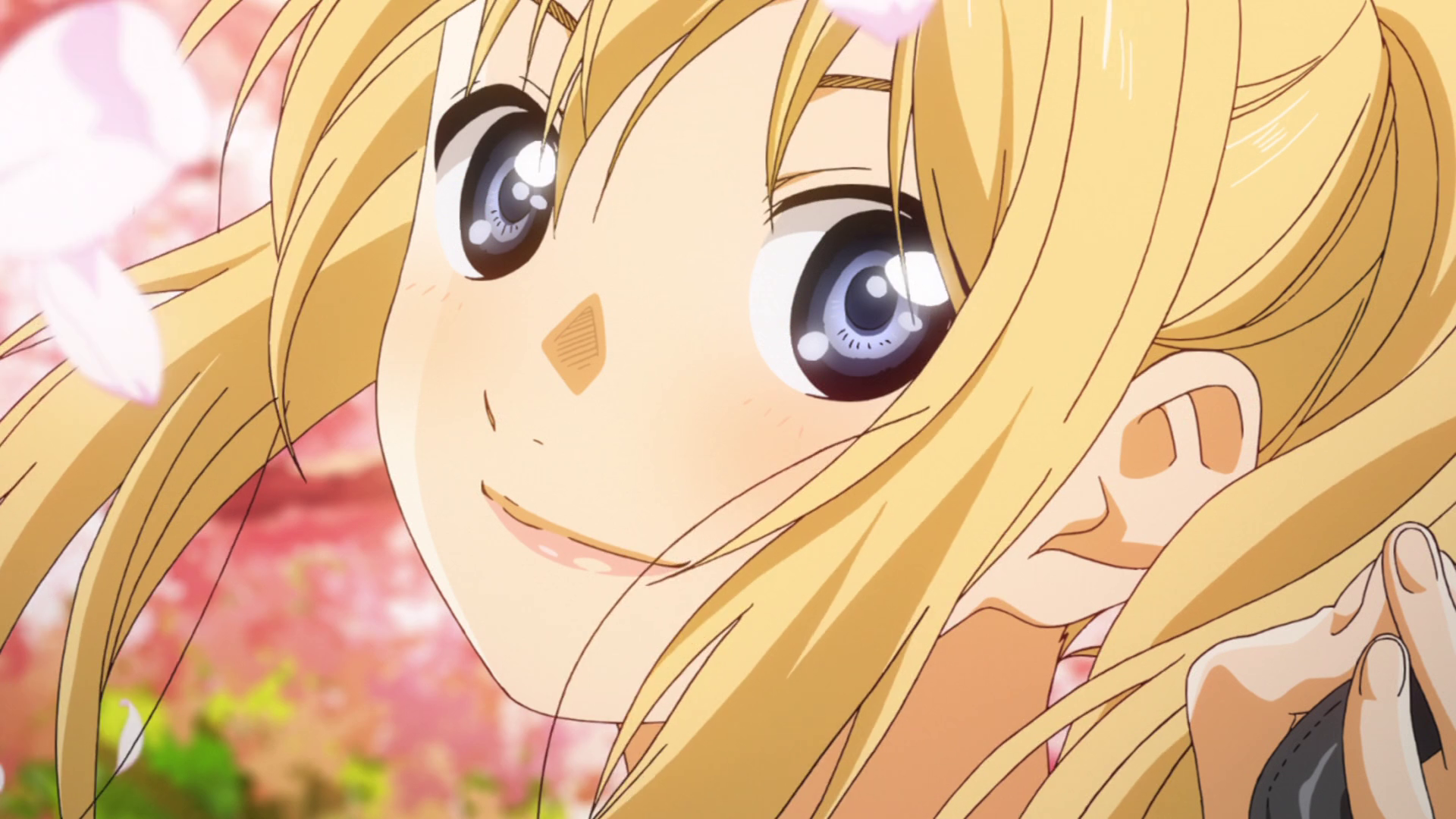
3.3. Motion detection
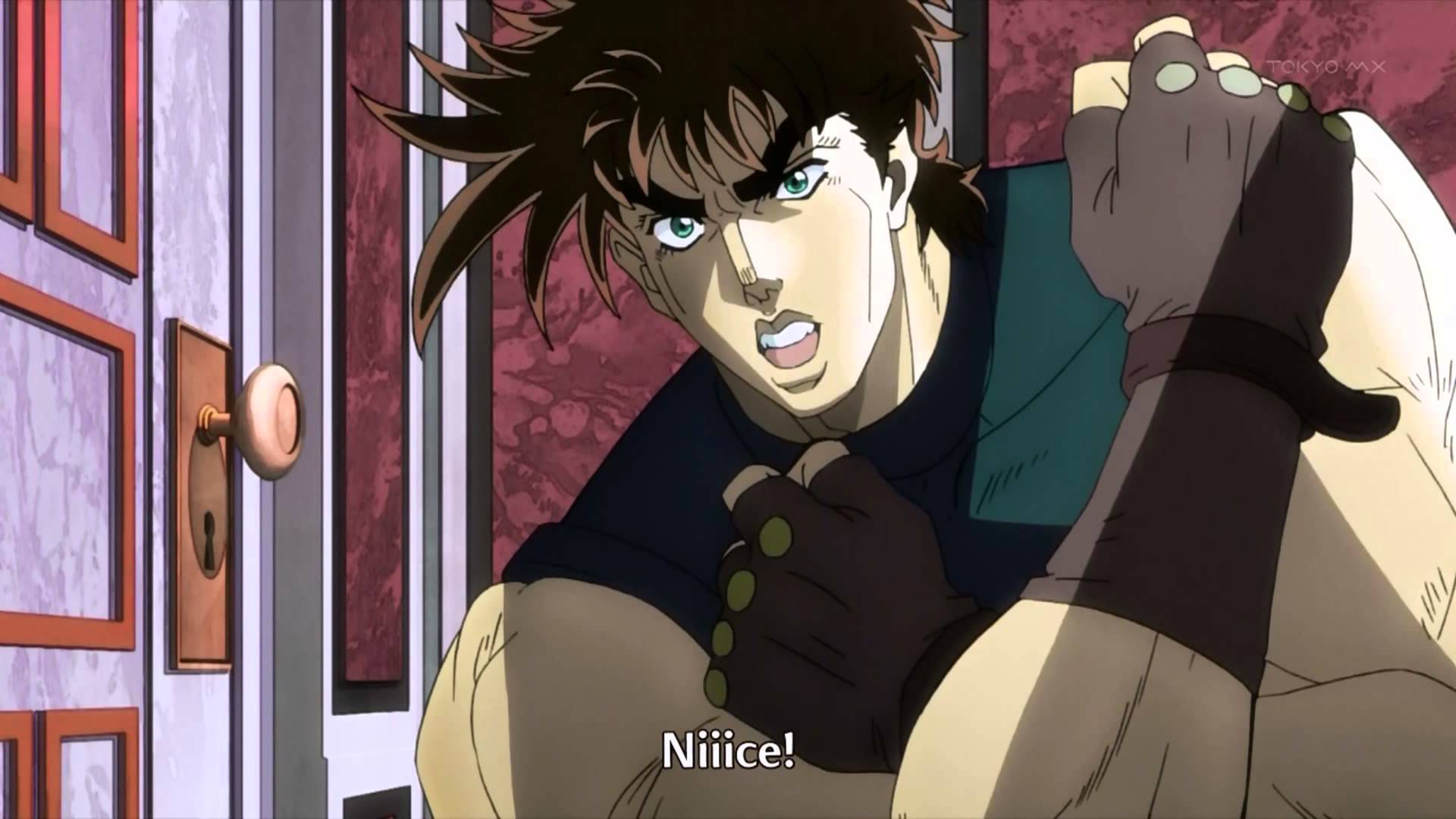
This programs alerts Iggy when Petshop arrives, it detects the drastic changes in the pixels. Take care of yourself Iggy, you have to help defeat Dio!
The input:
#include <iostream>
#include <cmath>
#include <opencv2/opencv.hpp>
using namespace cv;
using namespace std;
int main(int argc, char** argv){
Mat frame, img, hist, frame_hist;
int nbins = 64;
double compara;
float range[] = {0, 256};
const float *histrange = { range };
bool uniform = true;
bool acummulate = false;
VideoCapture cap("petshop.mp4");
if(!cap.isOpened()){
cout << "Erro abrindo o video!" <<endl;
return -1;
}
int histw = nbins, histh = nbins / 2;
Mat hist_img(histh, histw, CV_8UC1, Scalar(0, 0, 0));
cap >> frame;
cvtColor(frame, frame, CV_BGR2GRAY);
calcHist(&frame, 1, 0, Mat(), frame_hist, 1, &nbins, &histrange, uniform, acummulate);
normalize(frame_hist, frame_hist, 0, hist_img.rows, NORM_MINMAX, -1, Mat());
while(1){
cap >> img;
if (!img.data)
break;
cvtColor(img, img, CV_BGR2GRAY);
calcHist(&img, 1, 0, Mat(), hist, 1, &nbins, &histrange, uniform, acummulate);
normalize(hist, hist, 0, hist_img.rows, NORM_MINMAX, -1, Mat());
compara = compareHist(hist, frame_hist, CV_COMP_CORREL);
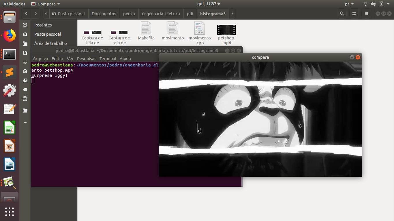
if (compara < 0.90)
cout << "Surpresa Iggy!" << endl;
cap >> frame;
cvtColor(frame, frame, CV_BGR2GRAY);
calcHist(&frame, 1, 0, Mat(), frame_hist, 1, &nbins, &histrange, uniform, acummulate);
normalize(hist, hist, 0, hist_img.rows, NORM_MINMAX, -1, Mat());
namedWindow("compara",WINDOW_AUTOSIZE);
imshow( "compara", img );
if(waitKey(30) >= 0)
break;
}
cap.release();
destroyAllWindows();
waitKey(0);
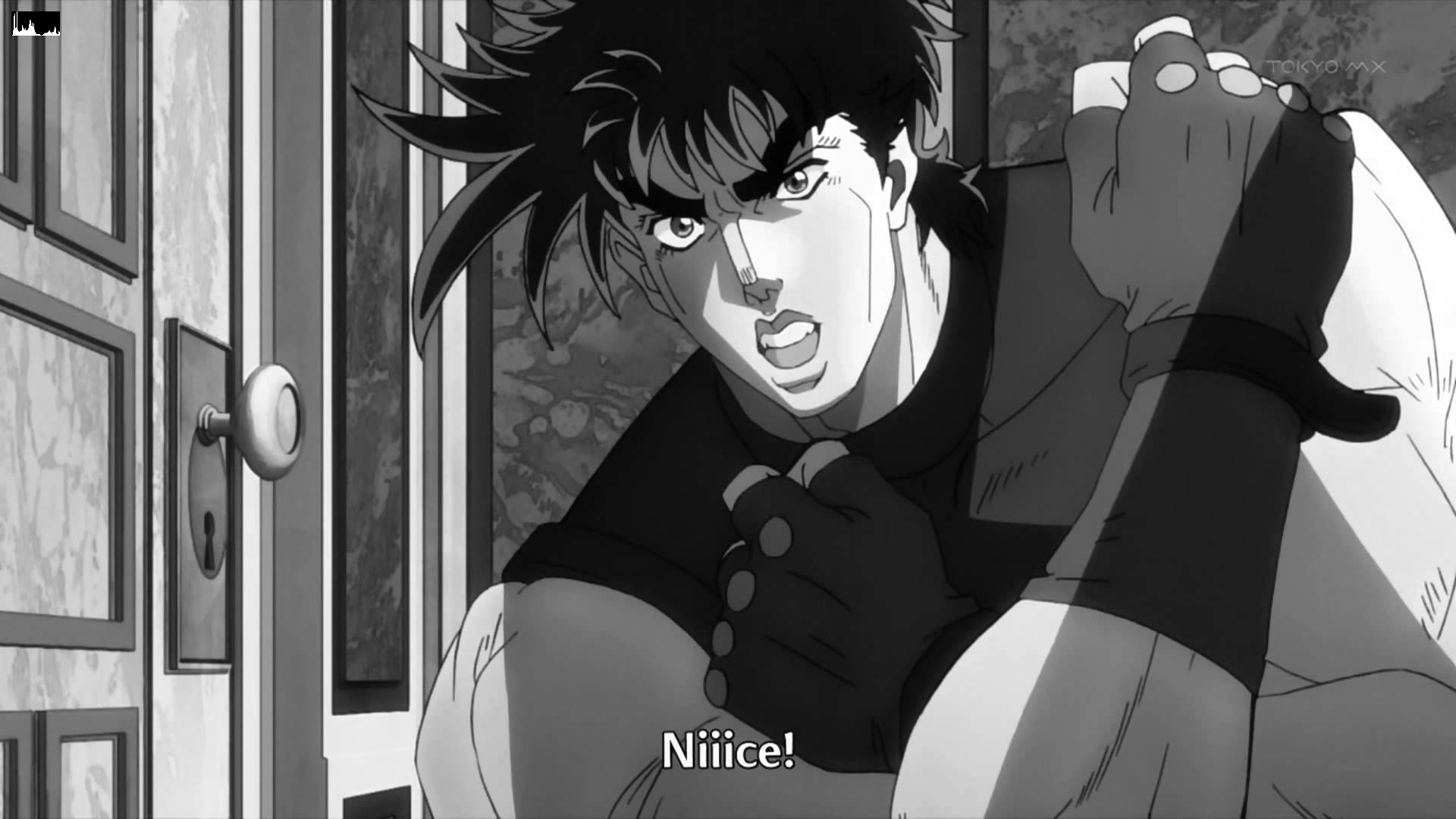
return 0;}Output:
It’s important to say that a compression happens in this process, since we are processing two frames in each loop.
4. Spatial-domain filtering I
4.1. Different kinds of filtering
After running the code, the image is filtered with different kernels, we can see it below.
Original image:
Grayscale:

#include <iostream>
#include <opencv2/opencv.hpp>

using namespace cv;
using namespace std;

void printmask(Mat &m) {
	for (int i = 0; i < m.size().height; i++) {
		for (int j = 0; j < m.size().width; j++) {
			cout << m.at<float>(i, j) << ",";
		}
		cout << endl;
	}
}

void menu() {
	cout << "\npressione a tecla para ativar o filtro: \n"
		"a - calcular modulo\n"
		"m - media\n"
		"g - gauss\n"
		"v - vertical\n"
		"h - horizontal\n"
		"l - laplaciano\n"
		"p - laplgauss\n"
		"esc - sair\n";
}

int main(int argvc, char** argv) {

	float media[] = { 1,1,1,
		1,1,1,
		1,1,1 };
	float gauss[] = { 1,2,1,
		2,4,2,
		1,2,1 };
	float vertical[] = { -1,0,1,
		-2,0,2,
		-1,0,1 };
	float horizontal[] = { -1,-2,-1,
		0,0,0,
		1,2,1 };
	float laplacian[] = { 0,-1,0,
		-1,4,-1,
		0,-1,0 };

	float laplgauss[] = {0,0,1,0,0,
		 0,1,2,1,0,
		1,2,-16,2,1,
		 0,1,2,1,0,
		 0,0,1,0,0};
	Mat img = imread("Kaori_Miyazono.png");
	if(!img.data)
    cout << "nao abriu bolhas.png" << endl;
	Mat  frame, frame32f, frameFiltered;
	Mat mask(3, 3, CV_32F), mask1;
	Mat result, result1;
	double width, height;
	int absolut;
	char key;

	width = img.cols;
	height = img.rows;
	std::cout << "largura=" << width << "\n";;
	std::cout << "altura =" << height << "\n";;

	namedWindow("filtroespacial", 1);

	mask = Mat(3, 3, CV_32F, media);
	scaleAdd(mask, 1 / 9.0, Mat::zeros(3, 3, CV_32F), mask1);
	swap(mask, mask1);
	absolut = 1;
	menu();
	for (;;) {
		cvtColor(img, frame, CV_BGR2GRAY);
		flip(frame, frame, 1);
		imshow("original", frame);

		frame.convertTo(frame32f, CV_32F);
		//imwrite("grayscale.jpg", frame);
		filter2D(frame32f, frameFiltered, frame32f.depth(), mask, Point(1, 1), 0);
		if (absolut) {
			frameFiltered = abs(frameFiltered);
		}
		frameFiltered.convertTo(result, CV_8U);
		imshow("filtroespacial", result);
		key = (char)waitKey(10);
		if (key == 27) break;
		switch (key) {
		case 'a':
			menu();
			absolut = !absolut;
			break;
		case 'm':
			menu();
			mask = Mat(3, 3, CV_32F, media);
			scaleAdd(mask, 1 / 9.0, Mat::zeros(3, 3, CV_32F), mask1);
			mask = mask1;
			printmask(mask);
			//imwrite("media.jpg", frameFiltered);
			break;
		case 'g':
			menu();
			mask = Mat(3, 3, CV_32F, gauss);
			scaleAdd(mask, 1 / 16.0, Mat::zeros(3, 3, CV_32F), mask1);
			mask = mask1;
			printmask(mask);
			//imwrite("gauss.jpg", frameFiltered);
			break;
		case 'h':
			menu();
			mask = Mat(3, 3, CV_32F, horizontal);
			printmask(mask);
			//imwrite("horizontal.jpg", frameFiltered);
			break;
		case 'v':
			menu();
			mask = Mat(3, 3, CV_32F, vertical);
			printmask(mask);
			//imwrite("vertical.jpg", frameFiltered);
			break;
		case 'l':
			menu();
			mask = Mat(3, 3, CV_32F, laplacian);
			printmask(mask);
			//imwrite("laplaciano.jpg", frameFiltered);
			break;

		case 'p':
			menu();
			mask = Mat(5, 5, CV_32F, laplgauss);
			printmask(mask);
			//imwrite("laplaciano_gaussiano.jpg", frameFiltered);
			break;
		default:
			break;
		}
	}
	return 0;
}
Gauss:
Media:
Horizontal:
Vertical:
Laplacian:
Laplacian + Gaussian:
We can see that using Laplacian + Gaussian filtering, the contours are now more well defined.
5. Spatial-domain filtering II
5.1. Tiltshift
Below we have the tilt-shift code, the algorithm simulates a change in focus of the image, partially blurring it.
This technique is very used in cinema industry, a recent example is the 2018 movie, Hereditary, where using the tilt-shift we have the footage looking like miniatures.
#include <iostream>
#include <opencv2/opencv.hpp>
#include <math.h>

using namespace cv;
using namespace std;

int main(int argvc, char** argv) {

  Mat image = imread("nausicaa.jpg");
  Mat gauss_image = Mat::zeros(image.rows, image.cols, CV_32FC3);
  Mat focus_image = Mat::zeros(image.rows, image.cols, CV_32FC3);
  Mat unfocus_image = Mat::zeros(image.rows, image.cols, CV_32FC3);
  Mat focus_mask = Mat(image.rows, image.cols, CV_32FC3, Scalar(0, 0, 0));
  Mat unfocus_mask = Mat(image.rows, image.cols, CV_32FC3, Scalar(1, 1, 1));
    Mat output = Mat::zeros(image.rows, image.cols, CV_32FC3);
    Vec3f funcion_output;

  float unfocus = 0.30;
  int decay = 50;
  int l1 = unfocus*image.rows;
  int l2 = image.rows - unfocus*image.rows;


  for (int i = 0; i < image.rows; i++) {
    for (int j = 0; j < image.cols; j++) {
      funcion_output[0] = (tanh((float(i - l1) / decay)) - tanh((float(i - l2) / decay))) / 2;
      funcion_output[1] = (tanh((float(i - l1) / decay)) - tanh((float(i - l2) / decay))) / 2;
      funcion_output[2] = (tanh((float(i - l1) / decay)) - tanh((float(i - l2) / decay))) / 2;
      focus_mask.at<Vec3f>(i, j) = funcion_output;
    }
  }

  unfocus_mask = unfocus_mask - focus_mask;

    image.convertTo(image, CV_32FC3);
  GaussianBlur(image, gauss_image, Size(7, 7), 0, 0);


    focus_image = image.mul(focus_mask);
  unfocus_image = gauss_image.mul(unfocus_mask);

  output = focus_image + unfocus_image;

  image.convertTo(image, CV_8UC3);
  output.convertTo(output, CV_8UC3);

    imshow("input", image);
  imshow("tiltshift", output);
  imwrite("nausicaa_tilt.jpg", output);

    waitKey();
    return 0;

}
Altough, the algorithm above works just with images.
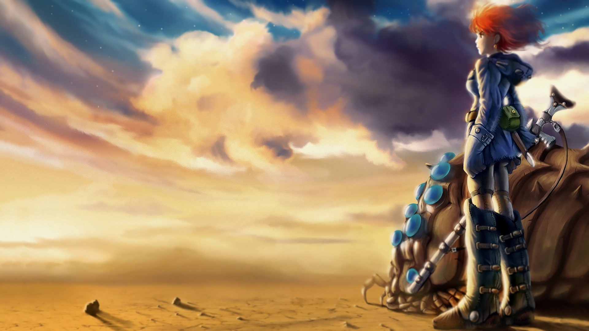
Input:

Output:
6. Frequence-domain filtering
6.1. Homomorphic filtering
The homomorphic filtering process is based on the principles of illuminace and reflectance. The illuminance represents slow spatial variations (low frequences), the reflectance represents fast spatial variations (high frequences). We take the fourier transform of the image and apply a sequential filter (modified version of gaussian filter) that attenuates low frequences and maintain high frequences (high-pass filter) and do the inverse fourier transform, this way, improving illuminance of image.
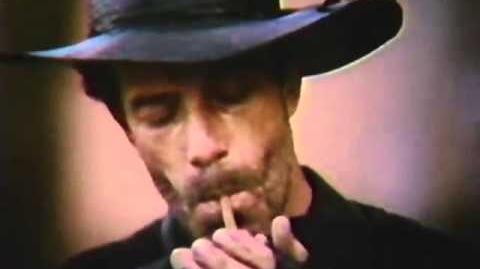
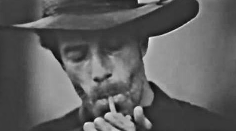
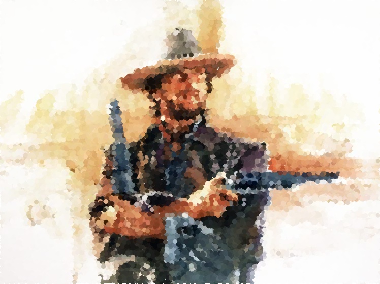
We can see the input below, Man with no name, Clint Eastwood’s character from A Fistful of Dollars movie:
Output:
Code below:
#include <iostream>
#include <opencv2/opencv.hpp>
#include <opencv2/imgproc/imgproc.hpp>

#define RADIUS 20

using namespace cv;
using namespace std;

// troca os quadrantes da imagem da DFT
void deslocaDFT(Mat& image ){
  Mat tmp, A, B, C, D;

  // se a imagem tiver tamanho impar, recorta a regiao para
  // evitar cópias de tamanho desigual
  image = image(Rect(0, 0, image.cols & -2, image.rows & -2));
  int cx = image.cols/2;
  int cy = image.rows/2;

  // reorganiza os quadrantes da transformada
  // A B   ->  D C
  // C D       B A
  A = image(Rect(0, 0, cx, cy));
  B = image(Rect(cx, 0, cx, cy));
  C = image(Rect(0, cy, cx, cy));
  D = image(Rect(cx, cy, cx, cy));

  // A <-> D
  A.copyTo(tmp);  D.copyTo(A);  tmp.copyTo(D);

  // C <-> B
  C.copyTo(tmp);  B.copyTo(C);  tmp.copyTo(B);
}

int main(int argc, char** argv){

  Mat imaginaryInput, complexImage, multsp;
  Mat padded, filter, mag;
  Mat image, imagegray, tmp;
  Mat_<float> realInput, zeros;
  vector<Mat> planos;

  if(argc!=2){
  exit(0);
  }
  image = imread(argv[1],CV_LOAD_IMAGE_GRAYSCALE);

  // valores ideais dos tamanhos da imagem
  // para calculo da DFT

  int dft_M, dft_N;

  // identifica os tamanhos otimos para
  // calculo do FFT
  dft_M = getOptimalDFTSize(image.rows);
  dft_N = getOptimalDFTSize(image.cols);

  // realiza o padding da imagem
  copyMakeBorder(image, padded, 0,
                 dft_M - image.rows, 0,
                 dft_N - image.cols,
                 BORDER_CONSTANT, Scalar::all(0));

  // parte imaginaria da matriz complexa (preenchida com zeros)
  zeros = Mat_<float>::zeros(padded.size());

  // prepara a matriz complexa para ser preenchida
  complexImage = Mat(padded.size(), CV_32FC2, Scalar(0));

  // a função de transferência (filtro frequencial) deve ter o
  // mesmo tamanho e tipo da matriz complexa
  filter = complexImage.clone();

  // cria uma matriz temporária para criar as componentes real
  // e imaginaria do filtro ideal
  tmp = Mat(dft_M, dft_N, CV_32F);

  // filtro homomorfico

  float gamah, gamal, c, D0;
  gamah = 150;
  gamal = 75;
  c = 15;
  D0 = 25;
  int M = dft_M;
  int N = dft_N;

for (int i = 0; i < dft_M; i++) {
    for (int j = 0; j < dft_N; j++) {
      tmp.at<float>(i, j) = (gamah - gamal)*(1.0 - exp(-1.0*(float)c*((((float)i - M / 2.0)*((float)i - M / 2.0) + ((float)j - N / 2.0)*((float)j - N / 2.0)) / (D0*D0)))) + gamal;
    }
  }

  // cria a matriz com as componentes do filtro e junta
  // ambas em uma matriz multicanal complexa
  Mat comps[]= {tmp, tmp};
  merge(comps, 2, filter);

    // limpa o array de matrizes que vao compor a
    // imagem complexa
    planos.clear();
    // cria a compoente real
    realInput = Mat_<float>(padded);
    // insere as duas componentes no array de matrizes
    planos.push_back(realInput);
    planos.push_back(zeros);

    // combina o array de matrizes em uma unica
    // componente complexa
    merge(planos, complexImage);

    // calcula o dft
    dft(complexImage, complexImage);

    // realiza a troca de quadrantes
    deslocaDFT(complexImage);

    // aplica o filtro frequencial
    mulSpectrums(complexImage,filter,complexImage,0);

    // limpa o array de planos
    planos.clear();
    // separa as partes real e imaginaria para modifica-las
    split(complexImage, planos);

    // recompoe os planos em uma unica matriz complexa
    merge(planos, complexImage);

    // troca novamente os quadrantes
    deslocaDFT(complexImage);


    // calcula a DFT inversa
    idft(complexImage, complexImage);

    // limpa o array de planos
    planos.clear();

    // separa as partes real e imaginaria da
    // imagem filtrada
    split(complexImage, planos);

    // normaliza a parte real para exibicao
    normalize(planos[0], planos[0], 0, 1, CV_MINMAX);
    imshow("filtrada", planos[0]);
    imshow("original", image);
    imwrite("papa.jpg", image);
    waitKey();

  return 0;
}
7. Pointillism
7.1. Pointillism art
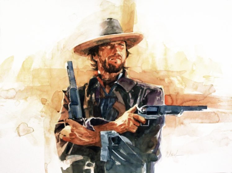
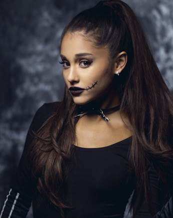
The program below do the pointillism in a RGB image, again we can see Clint:
Output:
Code:
#include <iostream>
#include <opencv2/opencv.hpp>
#include <fstream>
#include <iomanip>
#include <vector>
#include <algorithm>
#include <numeric>
#include <ctime>
#include <cstdlib>

using namespace std;
using namespace cv;

#define STEP 4
#define JITTER 3
#define RAIO 4

int top_slider = 10;
int top_slider_max = 200;

Mat image, border, frame, points, tmp, result;

void canny1(int, void *){
  Canny(image, border, top_slider, 3 * top_slider);
  imshow("canny", border);
}


int main(int argc, char** argv){
  vector<int> yrange;
  vector<int> xrange;
  int width, height;
  int x, y;
  int r, g, b;

  image= imread(argv[1]);

  srand(time(0));

  if(!image.data){
  cout << "nao abriu" << argv[1] << endl;
    cout << argv[0] << " imagem.jpg";
    exit(0);
  }

  width=image.size().width;
  height=image.size().height;

  xrange.resize(height/STEP);
  yrange.resize(width/STEP);

  iota(xrange.begin(), xrange.end(), 0);
  iota(yrange.begin(), yrange.end(), 0);

  for(uint i=0; i<xrange.size(); i++){
    xrange[i]= xrange[i]*STEP+STEP/2;
  }

  for(uint i=0; i<yrange.size(); i++){
    yrange[i]= yrange[i]*STEP+STEP/2;
  }

  points = Mat(height, width, CV_8UC3, Scalar(CV_RGB(255, 255, 255)));

  random_shuffle(xrange.begin(), xrange.end());

  for(auto i : xrange){
    random_shuffle(yrange.begin(), yrange.end());
    for(auto j : yrange){
      x = i+rand()%(2*JITTER)-JITTER+1;
      y = j+rand()%(2*JITTER)-JITTER+1;
      r = image.at<Vec3b>(x, y)[2];
      g = image.at<Vec3b>(x, y)[1];
      b = image.at<Vec3b>(x, y)[0];
      circle(points, cv::Point(y, x), RAIO, CV_RGB(r, g, b), -1, CV_AA);
    }
  }

  imshow("pontos", points);
  imwrite(argv[2], points);
  waitKey();

  return 0;
}
The program above basically goes through each pixel on image and draws a circle of radius 4 with same color and at the correspondent position, using a step of 4 (picks one pixel for each 4, in axis x and y).
8. Vector quantization with K-means
8.1. The K-means process
K-means is a quantization process that aims to sort N observations in K clusters.
In digital image processing, each observation corresponds to one pixel, and the clusters are the quantity of colors we want. We can sort each pixel from the aproximation with each centroid (one centroid for cluster), then, we take the mean distance of the samples in each cluster, crating new centroids positions. It’s a iterative process, this process happens until we don’t have more significative changes in centroids positions, finally, we can attribute one color for each cluster.
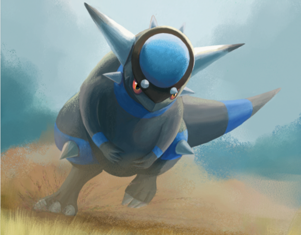
Input:
We can see the code below:
#include <opencv2/opencv.hpp>
#include <cstdlib>
using namespace cv;
int main( int argc, char** argv ){
int nClusters = 10;
Mat rotulos;
int nRodadas = 1;
int n = 2;
Mat centros;
if(argc!=12){
exit(0);
}
Mat img = imread( argv[1], CV_LOAD_IMAGE_COLOR);
Mat samples(img.rows * img.cols, 3, CV_32F);
for (int i = 0; i < 10; i++) {
for( int y = 0; y < img.rows; y++ ){
for( int x = 0; x < img.cols; x++ ){
for( int z = 0; z < 3; z++){
samples.at<float>(y + x*img.rows, z) = img.at<Vec3b>(y,x)[z];
}
}
}
kmeans(samples,
nClusters,
rotulos,
TermCriteria(CV_TERMCRIT_ITER|CV_TERMCRIT_EPS, 10000, 0.0001),
nRodadas,
KMEANS_RANDOM_CENTERS,
centros );
Mat rotulada( img.size(), img.type() );
for( int y = 0; y < img.rows; y++ ){
for( int x = 0; x < img.cols; x++ ){
int indice = rotulos.at<int>(y + x*img.rows,0);
rotulada.at<Vec3b>(y,x)[0] = (uchar) centros.at<float>(indice, 0);
rotulada.at<Vec3b>(y,x)[1] = (uchar) centros.at<float>(indice, 1);
rotulada.at<Vec3b>(y,x)[2] = (uchar) centros.at<float>(indice, 2);
}
}
imshow( "clustered image", rotulada );
imwrite(argv[n], rotulada);
n++;
waitKey( 0 );
}
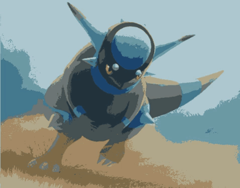
}In the program above, as requested by professor, we used the parameter KMEANS_RANDOM_CENTERS instead of KMEANS_PP_CENTERS, so, each Cluster initial position is randomized. It’s important to say that as we have random initial positions, we have differents outputs each time, for 10 rounds, we have 10 differents outputs, as is shown below.
Output:
BONUS:
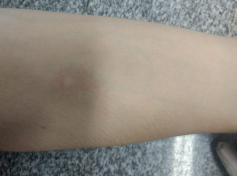
9. Case study - Prick Test
9.1 Allergy
Allergy is every kind of reaction from the body to a substance considered strange. Things of our day-to-day life can cause allergy, we call these things allergens. Sneezing, coryza, itchiness, hives, unwell and even glottal edema, which can lead person to obit can be consequences of an allergic reaction.
9.2 Prick test
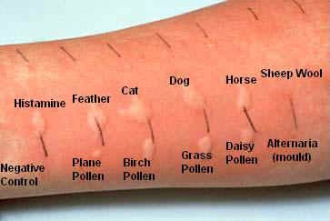
Prick test is an "in vivo" method (which is done in the body) that aims to detect allergens which the patient is sensible. This test detects inhalants and food sensitivities.
The test usually happens in the volar region of forearm or on in the back. A drop of negative control (usually saline, where is to happen absense of swelling) is dropped, also a drop of positive control (histamine), and drops of suspicious extracts, then, the punctures are aplyed. After waiting 15 minutes, the doctor can examine the size of the swell.
The swelling is measured in milimeters and assigned with up to 4 levels of allergy, marked with crosses.
The verification is done to the naked eye, with the aid of a ruler, here is where the digital images processing can aid. Nowadays this measurement is too subjective, some doctors don’t even use the ruler, and the help of softwere can make the detection more accurate and objective.
9.3 The process
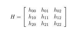
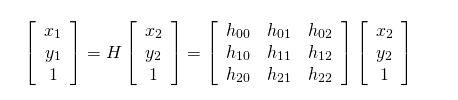
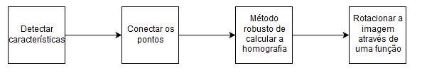
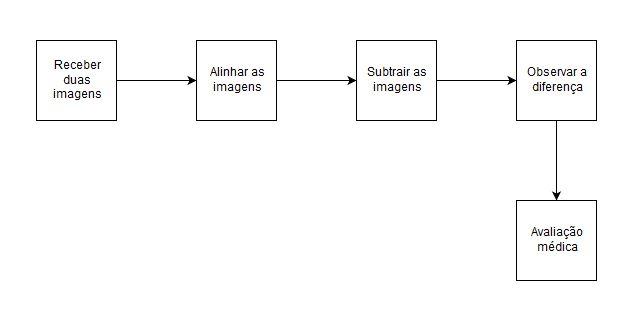
Our initial idea is basically subtract the image of patient’s arm before and after prick test, so the doctor could evaluate the result, maybe with auxilium of a digital ruler. Buf first we would need to align both images, homography could be a good solution to alignment, which relates two coordinates of images in same surface by a homography matrix H. Below we can see the Homography process and the block diagram of the process.
We may face difficulties, because of ilumination and distance, so we will need a referance, and maybe a support to arm and camera.
Below is the block diagram of the complete process.
9.4 Laboratory visit
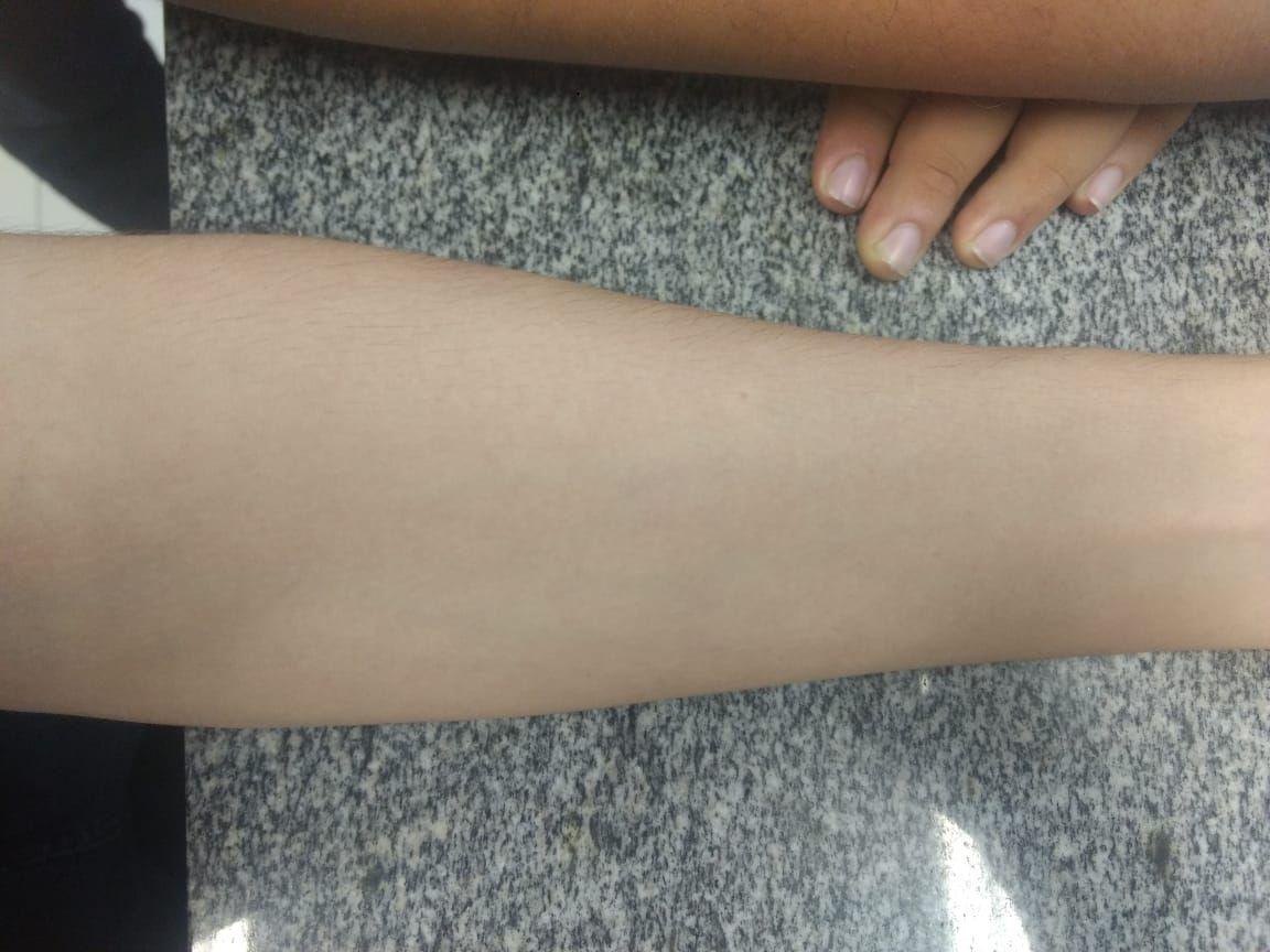
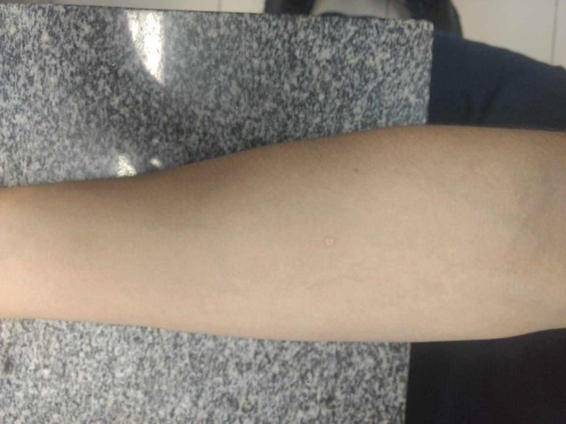
We had a reunion with proffessor Valéria Soraya de Faria Sales at HUOL (Hospital Universitário Honófrio Lopes) where she gave us informations about the prick test. She made an example of a prick test in my arm, we can see it below.
9.5 Future objectives
We have the goal to implement the algorithm, and use this kind of process in others skin problems, like cancer or urticaria.